Renderer performance metrics
7ca1c42 · 2026-07-11 ↗
Frame time alone cannot explain a Monte Carlo renderer. One method may trace more rays per sample but need fewer samples; another may generate cheap candidates and one expensive visibility ray. This commit records nested timing and statistical work through the same named-buffer system as rendered data.
Quantities recorded by the renderer
| Quantity | Question |
|---|---|
| Pass/phase time | Where is time spent? |
| Samples | How many estimator draws were accumulated? |
| Rays/candidates | How much physical or proposal work produced each draw? |
| Error/variance | How good is the current estimate? |
A renderer comparison should connect them by reporting the time required to reach a specified error threshold. Sample count alone measures estimator work, not execution cost. Frame time alone measures cost without image quality.
CUDA VolPT records the testing hardware separately from its performance results. The same separation is used here: hardware and build configuration define the measurement context; timings, work counts, and image error are the observations.
Variance of the pixel estimator
For luminance samples \(x_1,\ldots,x_n\), the sample mean is \(\bar x\). The unbiased sample variance is
\[s^2=\frac{1}{n-1}\sum_{i=1}^{n}(x_i-\bar x)^2.\]For independent samples, the estimated variance of the mean is
\[\widehat{\operatorname{Var}}[\bar x]=\frac{s^2}{n}.\]The implementation stores running \(\sum x_i\) and \(\sum x_i^2\), using
\[\sum_i(x_i-\bar x)^2=\sum_i x_i^2-n\bar x^2.\]This identity avoids retaining all samples. It can lose precision when the two terms are close; double precision and clamping tiny negative round-off values make the reported diagnostic more stable.
The independence condition is not automatic. Consecutive ordinary path-tracing samples can be independent when their random streams are independent and the scene is static. Temporal reservoir reuse deliberately correlates estimates across frames. In that case \(s^2/n\) is not generally an unbiased estimate of the variance of the mean because covariance terms are omitted:
\[\operatorname{Var}[\bar x] = \frac{1}{n^2} \left( \sum_i\operatorname{Var}[x_i] +2\sum_{i<j}\operatorname{Cov}[x_i,x_j] \right).\]The running statistic is still a useful noise indicator, but it must not be described as a complete uncertainty estimate for temporally correlated ReSTIR output. Independent repeated renders or correlation-aware estimators are needed for that claim.
RMSE against a reference
Given rendered pixels \(C_p\) and reference pixels \(R_p\),
\[\operatorname{RMSE} = \sqrt{\frac{1}{P}\sum_{p=1}^{P}\lVert C_p-R_p\rVert^2}.\]RMSE measures error to a chosen reference, not perceptual quality. Reference resolution, crop, color space, exposure, and alpha handling must match.
The notation \(\lVert C_p-R_p\rVert^2\) also needs an implementation
convention. It may mean the sum of squared linear-RGB channel errors, a mean
over channels, or luminance error. Those differ by scale and spectral
sensitivity. HdRestir benchmark metadata should state the convention so a
threshold such as 0.01 is interpretable.
The reference is itself an estimate unless it was computed analytically. Reference noise adds to measured error and creates a floor below which the test image cannot appear to converge. Increasing the reference sample count, using independent seeds, and storing its generation metadata reduce this problem.
Nested timing in parallel code
Summing a timer from every parallel worker measures aggregate CPU time, which can exceed wall time. The metrics system collects worker-local values and rescales or reports them within the parent wall-clock scope. Names and parent indices form a hierarchy:
IntegrationPass
├── BSDF sample
└── Direct light
    ├── NEE candidates
    ├── BSDF candidates
    └── resampling
Metrics are compiled behind a flag so measurement overhead is explicit.
Wall time and aggregate worker time have different interpretations:
| Measurement | Includes | Can exceed frame wall time? |
|---|---|---|
| Parent wall timer | elapsed duration including waits and scheduling | no |
| Sum of worker-local timers | CPU time attributed across all workers | yes |
| GPU timestamp | device interval between timestamp commands | independent CPU timeline |
| End-to-end frame time | host work, device work, synchronization, and handoff | no |
This commit implements CPU-side hierarchical attribution. A later GPU profiler would need device timestamps rather than assuming command submission time is kernel execution time.
Read how the timing tree is built
Metric storage
buffers.Add(kMetricTimingOutputName, sizeof(float), idx + 1);
buffers.Get<float>(kMetricTimingOutputName)[idx] = 0.0f;

buffers.Add(kMetricNameOutputName, sizeof(MetricNameEntry), idx + 1);
std::snprintf(
    buffers.Get<MetricNameEntry>(kMetricNameOutputName)[idx].Name,
    sizeof(MetricNameEntry::Name),
    "%s",
    std::string(name).c_str());

buffers.Add(kMetricParentOutputName, sizeof(std::size_t), idx + 1);
buffers.Get<std::size_t>(kMetricParentOutputName)[idx] = parent;
Index idx ties duration, display name, and parent together. A flat collection
of buffers can therefore encode the tree shown above without pass-specific
profiling objects.
Scope-based timers
ScopedMetricTimer::~ScopedMetricTimer()
{
    const float ms{
        std::chrono::duration<float, std::milli>(
            std::chrono::steady_clock::now() - _t0)
            .count()};
    _buffers.Get<float>(kMetricTimingOutputName)[_index] = ms;
}
The destructor runs for normal return and stack unwinding. This RAII pattern prevents an early return from leaving a metric open or requiring a duplicated “stop timer” call.
Concurrent worker accumulation
auto values{provider.GetChecked(name).As<float>()};
std::atomic_ref<float> counter{values[index]};
counter.fetch_add(ms, std::memory_order_relaxed);
Several pixels may finish the same phase concurrently. atomic_ref prevents
lost additions without changing the buffer layout. memory_order_relaxed is
sufficient because the operation needs atomic numeric accumulation, not a
happens-before relationship for other memory.
Wall-time attribution
float cpuSum{0.0f};
for (const auto &[name, ms] : metrics)
{
    cpuSum += ms;
}
const float scale{cpuSum > 0.0f ? wallMs / cpuSum : 0.0f};

// ...

for (const auto &[name, ms] : metrics)
{
    indices.push_back(RecordMetric(buffers, name, ms * scale, parent));
}
If four equally busy workers each report 10 ms, their sum is 40 ms even though the enclosing phase may take about 10 ms of wall time. Scaling preserves the relative subdivision while making the children add up to the measured parent. It is an attribution model, not a claim that the phases ran serially.
The scaling assumes the worker-local categories account for the useful work in the measured parent. Time spent outside them—scheduler overhead, cache misses between scopes, allocation, or synchronization—is distributed in proportion to the recorded categories. The displayed child values therefore answer “how should parent wall time be attributed using these samples?” rather than “how long did this code execute in isolation?”
When metrics are disabled, the macros compile away. This keeps “measurement off” a distinct build whose timing is not silently charged for atomic updates.
Measurement overhead and repeatability
atomic_ref<float>::fetch_add is safe for concurrent accumulation, but many
workers updating the same cache line can contend. Timers, string registration,
debug overlays, and buffer reads also perturb the program being measured. A
performance report should state whether metrics were enabled and should avoid
comparing a metrics-enabled pipeline with a metrics-disabled one.
A practical protocol is:
- warm shader compilation, scene loading, and one-time allocations;
- fix scene, camera, resolution, renderer settings, and seed policy;
- run several independent repetitions;
- record wall time, work counts, and error at regular checkpoints;
- report median and dispersion across repetitions;
- retain raw measurements in addition to the plotted image.
Thermal state, background load, CPU frequency policy, and GPU capture tools can change timings. They do not invalidate a measurement, but they belong in its environment description.
Reading convergence evidence
A convergence curve must identify the scene and camera, resolution, renderer revision and settings, random-seed policy, reference image, hardware, build configuration, error metric, and horizontal coordinate. A curve against sample count measures estimator efficiency but omits different per-sample costs. A curve against elapsed time includes those costs and is the relevant comparison when the goal is a better image within a fixed time.
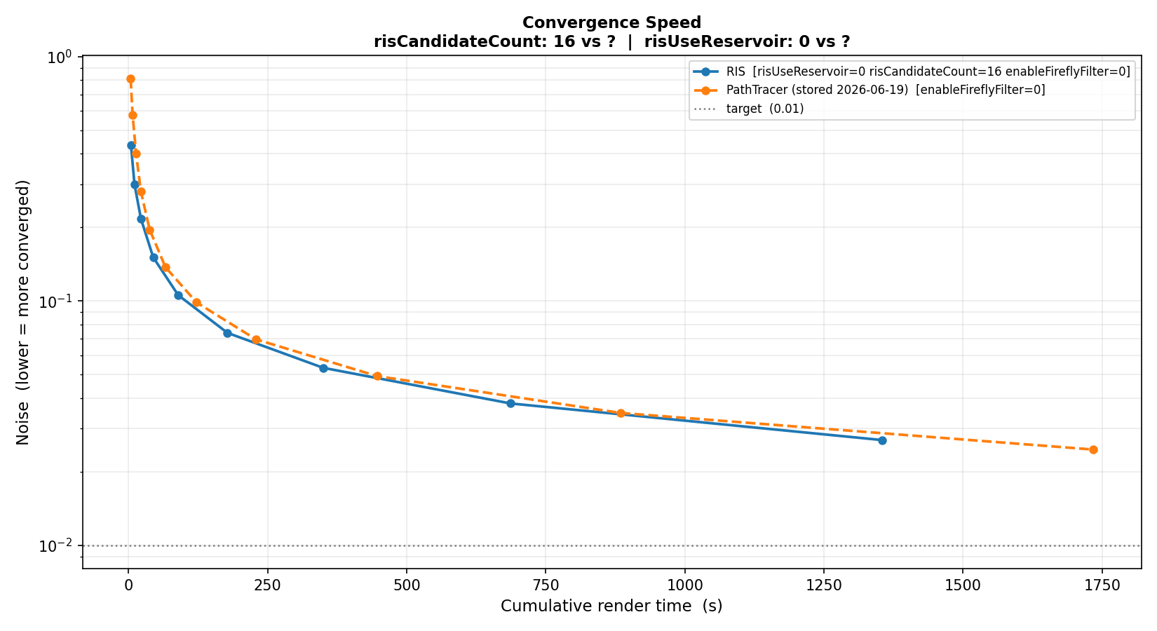
The final revision exposes ordinary path tracing and ReSTIR on both CPU and GPU. Separating estimator choice from execution backend requires a four-way comparison with a common scene, reference, exposure, stopping rule, and error metric.
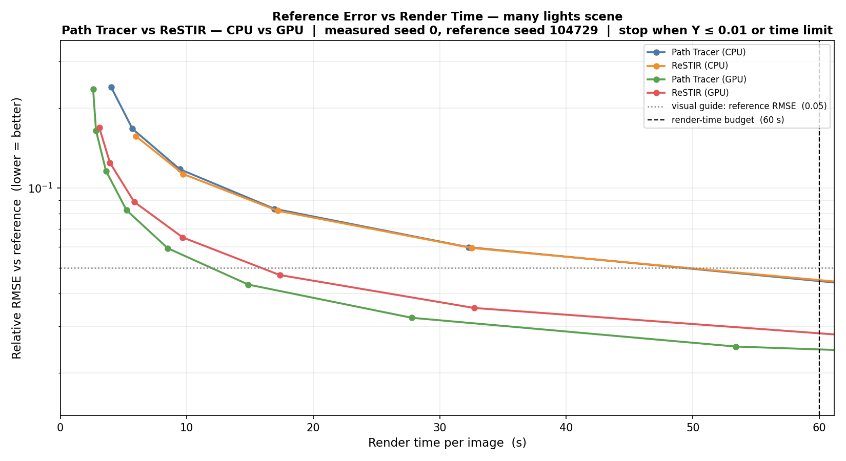
Many-light scenes emphasize candidate selection. A scene dominated by one large emitter or by long indirect paths can produce a different ordering, so the figures support only the configurations stated in their scopes.
Caption to keep: Candidate count should change proposal and resampling work; time-to-error determines whether that extra work is worthwhile.